Residuals and fitted values from model fit
Source:R/stat-fit-deviations.R, R/stat-fit-residuals.R
stat_fit_residuals.RdStatistic stat_fit_residuals fits a model and plots residuals vs.
x. Statistic stat_fit_deviations fits a model and and
highlighting residuals as segments in a y vs. x plot. Statistic
stat_fit_fitted plots the fitetd values vs. x.
Usage
stat_fit_deviations(
  mapping = NULL,
  data = NULL,
  geom = "segment",
  position = "identity",
  ...,
  orientation = NA,
  method = "lm",
  method.args = list(),
  n.min = 2L,
  formula = NULL,
  fit.seed = NA,
  na.rm = FALSE,
  show.legend = TRUE,
  inherit.aes = TRUE
)

stat_fit_fitted(
  mapping = NULL,
  data = NULL,
  geom = "point",
  position = "identity",
  orientation = NA,
  ...,
  method = "lm",
  method.args = list(),
  n.min = 2L,
  formula = NULL,
  fit.seed = NA,
  na.rm = FALSE,
  show.legend = FALSE,
  inherit.aes = TRUE
)

stat_fit_residuals(
  mapping = NULL,
  data = NULL,
  geom = "point",
  position = "identity",
  ...,
  orientation = NA,
  method = "lm",
  method.args = list(),
  n.min = 2L,
  formula = NULL,
  fit.seed = NA,
  resid.type = NULL,
  weighted = FALSE,
  na.rm = FALSE,
  show.legend = TRUE,
  inherit.aes = TRUE
)
Arguments
- mapping
The aesthetic mapping, usually constructed with
aes(). Only needs to be set at the layer level if you are overriding the plot defaults.- data
A layer specific dataset, only needed if you want to override the plot defaults.
- geom
The geometric object to use display the data
- position
The position adjustment to use for overlapping points on this layer.
- ...
other arguments passed on to
layer. This can include aesthetics whose values you want to set, not map. Seelayerfor more details.- orientation
character Either "x" or "y" controlling the default for
formula. The letter indicates the aesthetic considered the explanatory variable in the model fit.- method
function or character If character, "lm", "rlm", "lmrob", "lts", "gls", "ma", "sma", "segreg", "rq" or the name of a model fit function are accepted, possibly followed by the fit function's
methodargument separated by a colon (e.g."rlm:M"). If a function is different tolm(),rlm(),ltsReg(),gls(),ma,sma, it must have formal parameters namedformula,data, andweights. See Details.- method.args
named list with additional arguments. Not
dataorweightswhich are always passed through aesthetic mappings.- n.min
integer Minimum number of distinct values in the explanatory variable (on the rhs of formula) for fitting to the attempted.
- formula
a formula object. Using aesthetic names
xandyinstead of original variable names.- fit.seed
RNG seed argument passed to
set.seed(). Defaults toNA, indicating thatset.seed()should not be called.- na.rm
a logical indicating whether NA values should be stripped before the computation proceeds.
- show.legend
logical. Should this layer be included in the legends?
NA, the default, includes if any aesthetics are mapped.FALSEnever includes, andTRUEalways includes.- inherit.aes
If
FALSE, overrides the default aesthetics, rather than combining with them. This is most useful for helper functions that define both data and aesthetics and shouldn't inherit behaviour from the default plot specification, e.g.borders.- resid.type
character passed to
residuals()as argument fortype(defaults to"working"except ifweighted = TRUEwhen it is forced to"deviance").- weighted
logical If true weighted residuals will be returned.
Value
The returned value is always a data frame with the same number of
rows as the argument passed to data, except for the case failure of
the model fitting, in which case a data frame with no rows is returned. The
columns returned vary between the three statistics, and for each statistic
depending on the orientation..
To explore the values returned by statistics we suggest the use of
geom_debug_group(). Examples are shown below,
where one can also see in addition to the computed values the default
mapping of the fitted values to aesthetics xend and yend.
Details
stat_fit_deviations() can be used to highlight residuals as
segments in a plot of a fitted model prediction. This statistic returns the
original x and y values and the fitted y or x
values depending on the orientation, together with prior and
posterior weights.
stat_fit_fitted() can be used to highlight as points the fitted
values. This statistic returns the original x or y values
and the fitted y or x values depending on the
orientation.
stat_fit_residuals() plots residuals as points. It applies to the
fitted model object methods residuals() or
weighted.residuals() depending on the argument passed
to parameter weighted. This statistic returns the original x
and y values and residuals depending on the orientation,
together with prior and posterior weights.
Note
In the case of method = "rq" quantiles are fixed at tau =
0.5 unless method.args has length > 0. Parameter orientation
is redundant as it only affects the default for formula but is
included for consistency with ggplot2.
Prior and posterior weights
Two types of weights are possible: prior ones supplied in the call, and
posterior weights (called "robustness weights" in robust regression
methods) implicitly or explicitly used by fit methods to address
heterogeneity of error variance, including the presence of outlier
observations . Not all the supported methods accepts prior weights and
gls() returns posterior weights that are not in 0..1 like in the
case of most other fits. When not accessible weights are set to 1 when
known to be equal to 1, which is the most frequent case, or to NA
otherwise.
How weights are applied to residuals depends on the method used to fit the model. For ordinary least squares (OLS), weights are applied to the squares of the residuals, so the weighted residuals are obtained by multiplying the "deviance" residuals by the square root of the weights. When residuals are penalized differently to fit a model, the weighted residuals need to be computed accordingly.
Variables returned by stat_fit_residuals()
- x
x coordinates of observations
- y
y coordinates of observations
- x.resid
x residuals from fitted values
- y.resid
y residuals from fitted values
- weights
the weights passed as input to
lm(),rlm(),lmrob(), or to other model fit functions using aesthetic weight. More generally the value returned by methodweights()applied to the model fit object- robustness.weights
the "weights" of the applied minimization criterion relative to those of OLS in
rlm()orlmrob()or the divisor weights fromgls(),lme()ornlme()
Variables returned by stat_fit_deviations()
- x
x coordinates of observations
- y
y coordinates of observations
- x.fitted
x coordinates of fitted values
- y.fitted
y coordinates of fitted values
- weights
the weights passed as input to
lm(),rlm(), orlmrob(), using aesthetic weight. More generally the value returned byweights()- robustness.weights
the "weights" of the applied minimization criterion relative to those of OLS in
rlm(), orlmrob()
Variables returned by stat_fit_fitted()
- x
x coordinates of observations or fitted
- y
y coordinates of observations or fitted
Model formula and model fitting
A ggplot statistic receives as data a data frame that is not the one
passed as argument by the user, but instead a data frame with the variables
mapped to aesthetics. In stat_poly_eq() the compute function is
applied by group, each call "seeing" the subset of data for an
individual group. As supported models are for regression lines,
variables mapped to x and y should both be continuous, i.e.,
numeric or date time and model formulas defined using x and y
as variable names.
The interpretation of the argument passed to formula is enhanced
compared to stat_smooth(). Formulas with x as explanatory
variable work as in stat_smooth() but formulas with y as
explanatory variable are also accepted. orientation is set
automatically based on which explanatory variable appears in the formula.
Spline-based smoothers are only partially supported.
Model fit methods supported
Several model fit functions are supported explicitly (see tables), and some
of their differences smoothed out. Compatibility is checked late, based on
the class of the returned fitted model object. This makes it possible to
use wrapper functions that do model selection or other adjustments to the
fit procedure on a per panel or per group basis. Moreover, if the value
returned as model fit object is NULL or NA, plotting is
skipped on a per group within panel basis.
In the case of fitted model objects of classes not explicitly supported, an attempt is made to find the usual accessors and/or fitted object members, and if found, either complete or partial support is frequently achieved. In this case a message is issued encouraging users to check the validity of the values extracted as the structure of fitted model objects belonging to different classes and the values returned by their accessors can vary, potentially resulting in decoding errors leading to the return of wrong values for estimates.
The argument to parameter method can be either the name of a
function object, possibly using double colon notation in case its package
is not attached, or a character string matching the function name for
functions in the search path. This approach makes it possible to support
model fit functions that are not dependencies of 'ggpmisc'. Either by
attaching the package where the function is defined and passing it by name
or as string, or using double colon notation when passing the name of the
function.
User-defined functions can be passed as argument to parameter method
as long as they have parameters formula, data subset
and possibly weights. Additional arguments can be passed to any
method as a named list through parameter method.args. As in
stat_smooth() prior weights are
passed to the model fit functions' weights (plural!) parameter by
mapping a numeric variable to plot aesthetic weight (singular!).
Tables 1 lists natively supported model fit functions, with the caveat that only some 'broom' methods' specializations have been actually tested with statistics from 'ggpmisc'. In addition, the statistics based on 'broom' methods require the user to tailor their behaviour by passing additional arguments in the call and occasionally some detective work to find out the names of variables in the returned data frame as these names are set by methods from 'broom'.
Table 1. Model fit methods supported by the different statistics available in package 'ggpmisc'. Column \(f\) indicates whether computations are done by group (G) or by plot panel (P).
| Statistic | \(f\) | Supported model fit methods |
stat_poly_line() | G | "lm", "rlm", "lts", "sma", "ma", "gls", others with methods predict() or fitted() |
stat_poly_eq() | G | "lm", "rlm", "lts", "sma", "ma", "gls", others with needed accesors |
stat_quant_line() | G | "rq", "rqss" |
stat_quant_band() | G | "rq", "rqss" |
stat_quant_eq() | G | "rq", "rqss" |
stat_ma_line() | G | "SMA", "MA", "RMA", "OLS" |
stat_ma_eq() | G | "SMA", "MA", "RMA", "OLS" |
stat_fit_residuals() | G | "lm", "rlm", "lts", "sma", "ma", "gls", "rq", "rqss" others with method residuals() |
stat_fit_fitted() | G | "lm", "rlm", "lts", "gls", "rq", "rqss" others with method fitted() |
stat_fit_deviations() | G | "lm", "rlm", "lts", "gls", "rq", "rqss" others with methods fitted() and weights() |
stat_fit_augment() | G | any with 'broom' method augment() |
stat_fit_glance() | G | any with 'broom' method glance() |
stat_fit_tidy() | G | any with 'broom' method tidy() |
stat_fit_tb() | P | any with 'broom' method tidy() |
The single colon notation is based on parsing
the name and is available when passing the name of the fit method as a
character string. In a string such as "head:tail" the "head" gives the name
of the model fit function and the "tail" gives the argument to pass it's
method parameter. This is only a convenience, as method.args
can be also used. In some methods, i.e., splines, the default
formula = y ~ x needs to be overridden by the user.
Table 2 lists the correspondence of pre-defined method names to model fit method functions. As mentioned above, these are only a subset of the model fit methods that are expected to work. When using these names there is no need for users to attach additional packages but the packages must be available (installed).
Table 2. Available predefined method names, the model fit functions
they call, the packages where the functions reside, the class of the
returned fitted model object and the arguments that can be
passed to their method parameter using single colon notation.
| Predefined method names | Model fit methods | R package | Object class |
| "lm", "lm:qr" | lm() | 'stats' | "lm" |
| "rlm", "rlm:M", "rlm:MM" | rlm() | 'MASS' | "rlm" ("lm") |
| "lts", "ltsReg" | ltsReg() | 'robustbase' | "lts" |
| "ma", "sma", "sma:SMA", "sma:MA", "sma:OLS" | sma() | 'smatr' | "ma" or "sma" |
| "gls", "gls:REML", "gls:ML" | gls() | 'nlme' | "gls" |
| "rq", "rq:sfn", "rq:sfnc", "rq:lasso" | rq() | 'quantreg' | "rq" |
| "rqss", "rqss:sfn", "rqss:sfnc", "rqss:lasso" | rqss() | 'quantreg' | "rqss" |
| "SMA", "MA", "RMA", "OLS" | lmodel2() | 'lmodel2' | ("list") |
See also
Other 'ggpmisc' statistics for model fits:
stat_distrmix_eq(),
stat_fit_glance(),
stat_fit_tb(),
stat_fit_tidy(),
stat_ma_eq(),
stat_poly_eq(),
stat_quant_band()
Aesthetics
stat_fit_residuals() understands the following aesthetics. Required aesthetics are displayed in bold and defaults are displayed for optional aesthetics:
| • | x | |
| • | y | |
| • | group | → inferred |
stat_fit_deviations() understands the following aesthetics. Required aesthetics are displayed in bold and defaults are displayed for optional aesthetics:
| • | x | |
| • | y | |
| • | group | → inferred |
| • | xend | → after_stat(x.fitted) |
| • | yend | → after_stat(y.fitted) |
stat_fit_fitted() understands the following aesthetics. Required aesthetics are displayed in bold and defaults are displayed for optional aesthetics:
| • | x | |
| • | y | |
| • | group | → inferred |
Learn more about setting these aesthetics in vignette("ggplot2-specs").
Examples
# generate artificial data
set.seed(4321)
x <- 1:100
y <- (x + x^2 + x^3) + rnorm(length(x), mean = 0, sd = mean(x^3) / 4)
my.data <- data.frame(x, y)
# give a name to a formula
my.formula <- y ~ poly(x, 3, raw = TRUE)
my.y.formula <- x ~ poly(y, 3, raw = TRUE)
# plot residuals from linear model
ggplot(my.data, aes(x, y)) +
stat_poly_line(method = "lm", formula = my.formula) +
stat_fit_deviations(method = "lm", formula = my.formula, colour = "red") +
geom_point()
 # plot residuals from linear model with y as explanatory variable
ggplot(my.data, aes(x, y)) +
stat_poly_line(method = "lm", formula = my.y.formula) +
stat_fit_deviations(method = "lm", formula = my.y.formula, colour = "red") +
geom_point()
# plot residuals from linear model with y as explanatory variable
ggplot(my.data, aes(x, y)) +
stat_poly_line(method = "lm", formula = my.y.formula) +
stat_fit_deviations(method = "lm", formula = my.y.formula, colour = "red") +
geom_point()
 # plot robust regression
ggplot(my.data, aes(x, y)) +
stat_poly_line(formula = my.formula, method = "rlm") +
stat_fit_deviations(formula = my.formula, method = "rlm", colour = "red") +
geom_point()
# plot robust regression
ggplot(my.data, aes(x, y)) +
stat_poly_line(formula = my.formula, method = "rlm") +
stat_fit_deviations(formula = my.formula, method = "rlm", colour = "red") +
geom_point()
 # plot robust regression with weights indicated by colour
my.data.outlier <- my.data
my.data.outlier[6, "y"] <- my.data.outlier[6, "y"] * 5
ggplot(my.data.outlier, aes(x, y)) +
stat_poly_line(method = MASS::rlm, formula = my.formula) +
stat_fit_deviations(formula = my.formula, method = "rlm",
mapping = aes(colour = after_stat(robustness.weights)),
show.legend = TRUE) +
scale_color_gradient(low = "red", high = "blue", limits = c(0, 1),
guide = "colourbar") +
geom_point()
# plot robust regression with weights indicated by colour
my.data.outlier <- my.data
my.data.outlier[6, "y"] <- my.data.outlier[6, "y"] * 5
ggplot(my.data.outlier, aes(x, y)) +
stat_poly_line(method = MASS::rlm, formula = my.formula) +
stat_fit_deviations(formula = my.formula, method = "rlm",
mapping = aes(colour = after_stat(robustness.weights)),
show.legend = TRUE) +
scale_color_gradient(low = "red", high = "blue", limits = c(0, 1),
guide = "colourbar") +
geom_point()
 # plot quantile regression (= median regression)
ggplot(my.data, aes(x, y)) +
stat_quantile(formula = my.formula, quantiles = 0.5) +
stat_fit_deviations(formula = my.formula, method = "rq", colour = "red") +
geom_point()
# plot quantile regression (= median regression)
ggplot(my.data, aes(x, y)) +
stat_quantile(formula = my.formula, quantiles = 0.5) +
stat_fit_deviations(formula = my.formula, method = "rq", colour = "red") +
geom_point()
 # plot quantile regression (= "quartile" regression)
ggplot(my.data, aes(x, y)) +
stat_quantile(formula = my.formula, quantiles = 0.75) +
stat_fit_deviations(formula = my.formula, colour = "red",
method = "rq", method.args = list(tau = 0.75)) +
geom_point()
# plot quantile regression (= "quartile" regression)
ggplot(my.data, aes(x, y)) +
stat_quantile(formula = my.formula, quantiles = 0.75) +
stat_fit_deviations(formula = my.formula, colour = "red",
method = "rq", method.args = list(tau = 0.75)) +
geom_point()
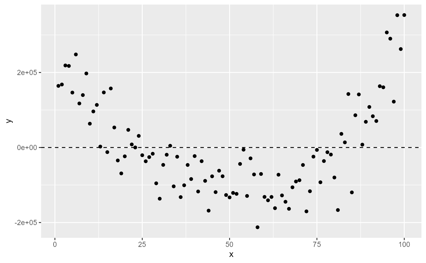
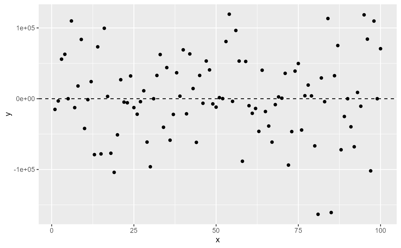
 # plot residuals from linear model
ggplot(my.data, aes(x, y)) +
geom_hline(yintercept = 0, linetype = "dashed") +
stat_fit_residuals(formula = my.formula)
# plot residuals from linear model
ggplot(my.data, aes(x, y)) +
geom_hline(yintercept = 0, linetype = "dashed") +
stat_fit_residuals(formula = my.formula)
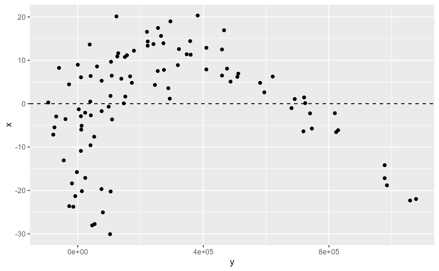
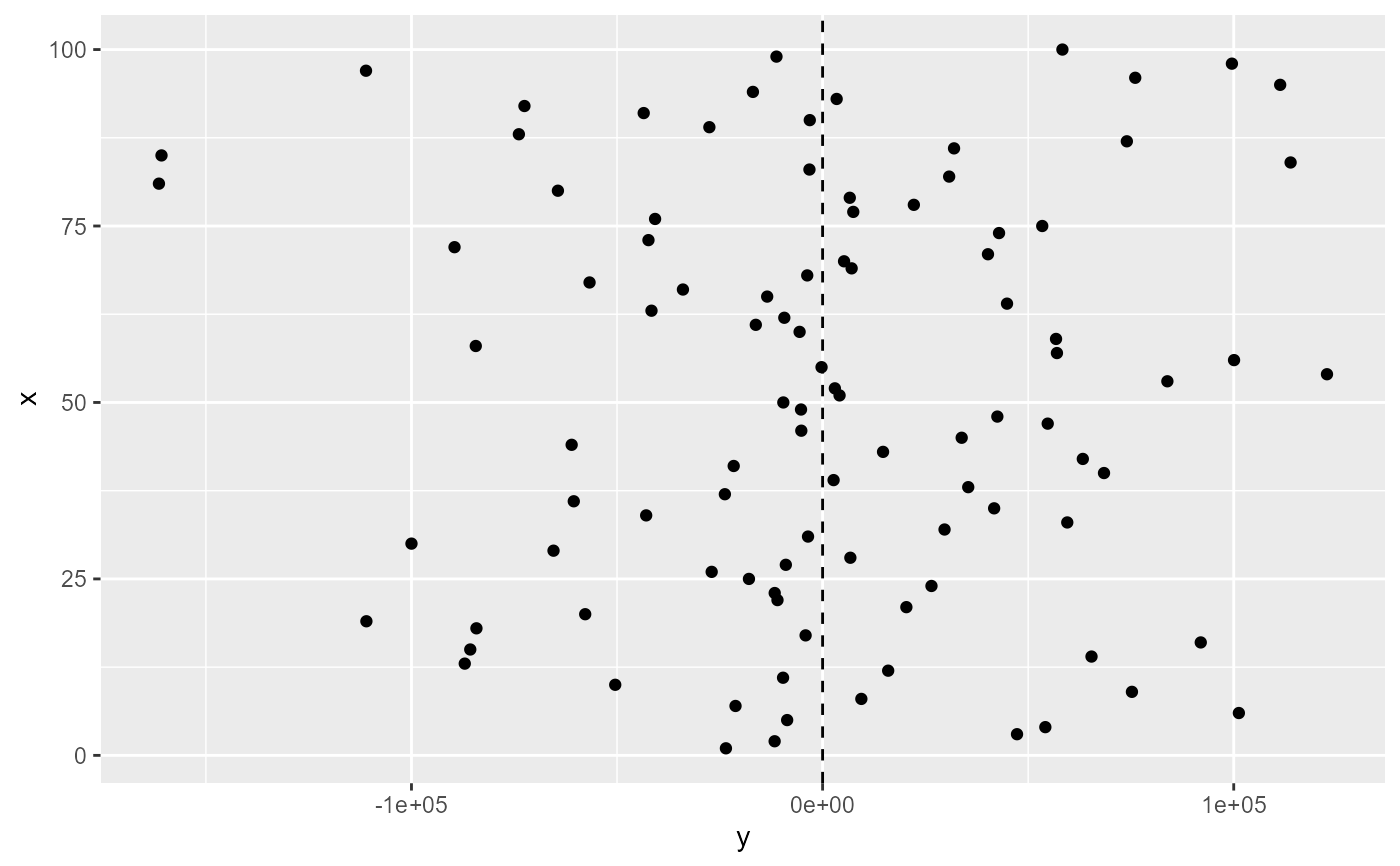
 # plot residuals from linear model with y as explanatory variable
ggplot(my.data, aes(x, y)) +
geom_vline(xintercept = 0, linetype = "dashed") +
stat_fit_residuals(formula = my.y.formula) +
coord_flip()
# plot residuals from linear model with y as explanatory variable
ggplot(my.data, aes(x, y)) +
geom_vline(xintercept = 0, linetype = "dashed") +
stat_fit_residuals(formula = my.y.formula) +
coord_flip()
 ggplot(my.data, aes(x, y)) +
geom_hline(yintercept = 0, linetype = "dashed") +
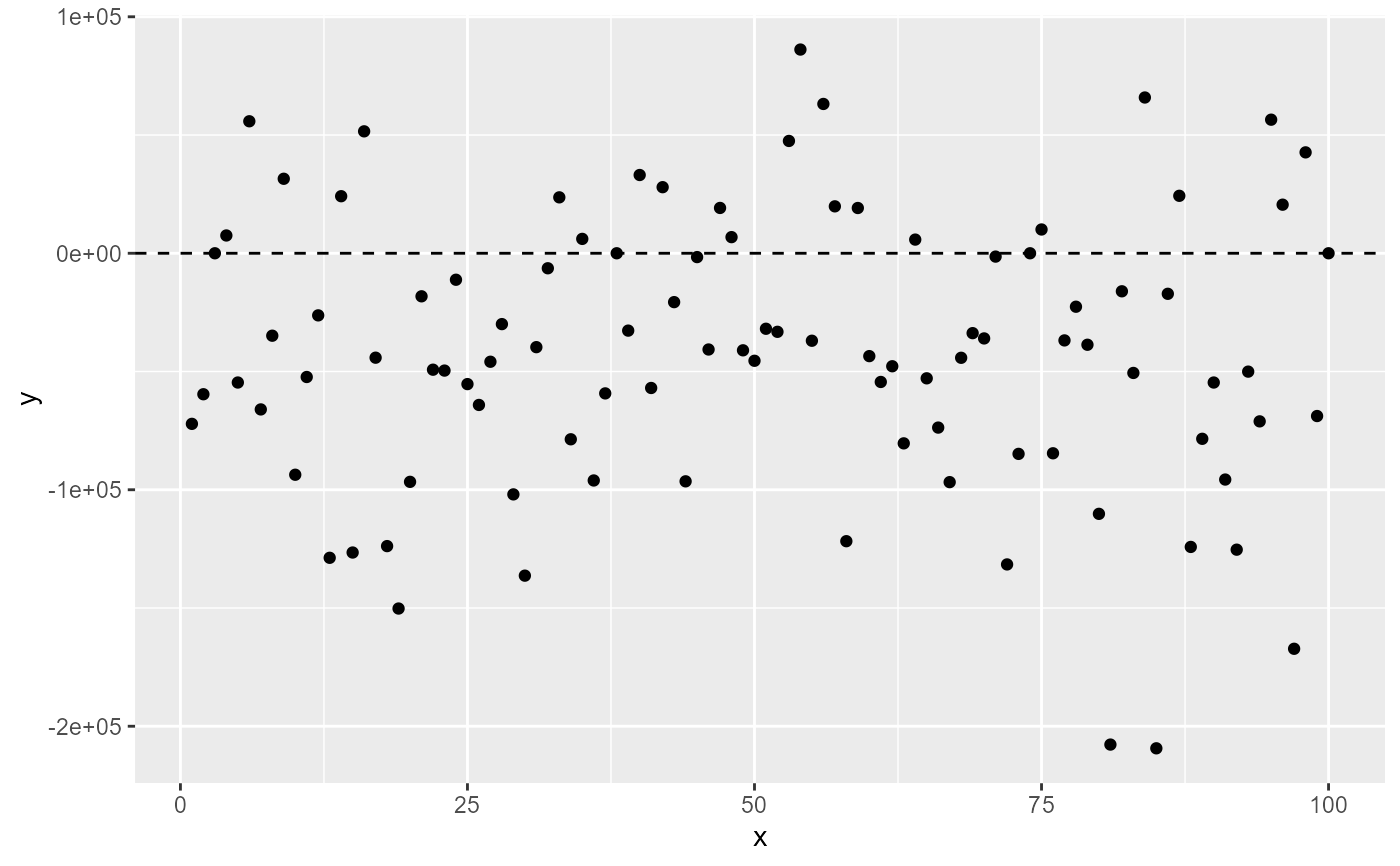
stat_fit_residuals(formula = my.formula, resid.type = "response")
ggplot(my.data, aes(x, y)) +
geom_hline(yintercept = 0, linetype = "dashed") +
stat_fit_residuals(formula = my.formula, resid.type = "response")
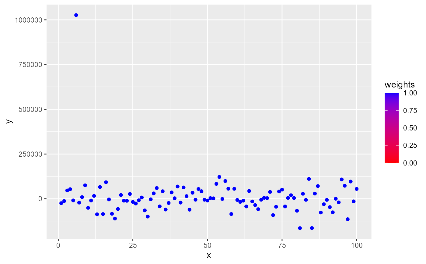
 # plot residuals with weights indicated by colour
my.data.outlier <- my.data
my.data.outlier[6, "y"] <- my.data.outlier[6, "y"] * 5
ggplot(my.data.outlier, aes(x, y)) +
stat_fit_residuals(formula = my.formula, method = "rlm",
mapping = aes(colour = after_stat(robustness.weights)),
show.legend = TRUE) +
scale_color_gradient(low = "red", high = "blue", limits = c(0, 1),
guide = "colourbar")
# plot residuals with weights indicated by colour
my.data.outlier <- my.data
my.data.outlier[6, "y"] <- my.data.outlier[6, "y"] * 5
ggplot(my.data.outlier, aes(x, y)) +
stat_fit_residuals(formula = my.formula, method = "rlm",
mapping = aes(colour = after_stat(robustness.weights)),
show.legend = TRUE) +
scale_color_gradient(low = "red", high = "blue", limits = c(0, 1),
guide = "colourbar")
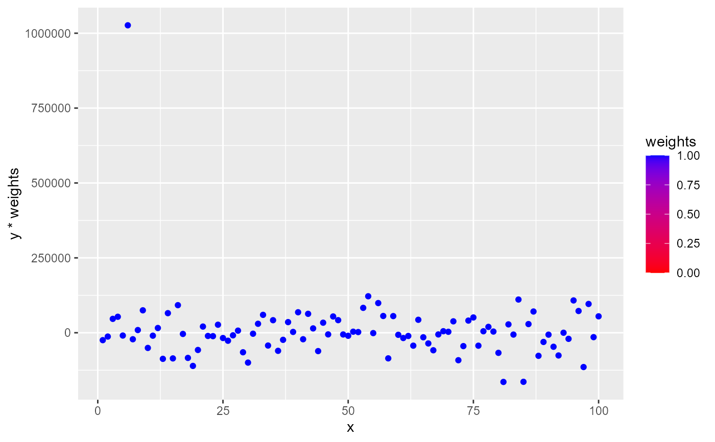
 # plot weighted residuals with weights indicated by colour
ggplot(my.data.outlier) +
stat_fit_residuals(formula = my.formula, method = "rlm",
mapping = aes(x = x,
y = stage(start = y, after_stat = y * weights),
colour = after_stat(robustness.weights)),
show.legend = TRUE) +
scale_color_gradient(low = "red", high = "blue", limits = c(0, 1),
guide = "colourbar")
# plot weighted residuals with weights indicated by colour
ggplot(my.data.outlier) +
stat_fit_residuals(formula = my.formula, method = "rlm",
mapping = aes(x = x,
y = stage(start = y, after_stat = y * weights),
colour = after_stat(robustness.weights)),
show.legend = TRUE) +
scale_color_gradient(low = "red", high = "blue", limits = c(0, 1),
guide = "colourbar")
 # inspecting the returned data
gginnards.installed <- requireNamespace("gginnards", quietly = TRUE)
if (gginnards.installed)
library(gginnards)
# plot, using geom_debug_group() to explore the after_stat data
if (gginnards.installed)
ggplot(my.data, aes(x, y)) +
stat_fit_deviations(formula = my.formula,
geom = "debug_group")
# inspecting the returned data
gginnards.installed <- requireNamespace("gginnards", quietly = TRUE)
if (gginnards.installed)
library(gginnards)
# plot, using geom_debug_group() to explore the after_stat data
if (gginnards.installed)
ggplot(my.data, aes(x, y)) +
stat_fit_deviations(formula = my.formula,
geom = "debug_group")
 #> [1] "PANEL 1; group(s) -1; 'draw_function()' input 'data' (head):"
#> x y x.fitted y.fitted weights robustness.weights hjust PANEL group
#> 1 1 -27205.450 1 -3691.7638 1 1 0 1 -1
#> 2 2 -14242.651 2 -2578.9186 1 1 0 1 -1
#> 3 3 45790.918 3 -1498.5419 1 1 0 1 -1
#> 4 4 53731.420 4 -443.8109 1 1 0 1 -1
#> 5 5 -8028.578 5 592.0973 1 1 0 1 -1
#> 6 6 102863.943 6 1616.0056 1 1 0 1 -1
#> xend yend orientation
#> 1 1 -3691.7638 x
#> 2 2 -2578.9186 x
#> 3 3 -1498.5419 x
#> 4 4 -443.8109 x
#> 5 5 592.0973 x
#> 6 6 1616.0056 x
if (gginnards.installed)
ggplot(my.data.outlier, aes(x, y)) +
stat_fit_deviations(formula = my.formula, method = "rlm",
geom = "debug_group")
#> [1] "PANEL 1; group(s) -1; 'draw_function()' input 'data' (head):"
#> x y x.fitted y.fitted weights robustness.weights hjust PANEL group
#> 1 1 -27205.450 1 -3691.7638 1 1 0 1 -1
#> 2 2 -14242.651 2 -2578.9186 1 1 0 1 -1
#> 3 3 45790.918 3 -1498.5419 1 1 0 1 -1
#> 4 4 53731.420 4 -443.8109 1 1 0 1 -1
#> 5 5 -8028.578 5 592.0973 1 1 0 1 -1
#> 6 6 102863.943 6 1616.0056 1 1 0 1 -1
#> xend yend orientation
#> 1 1 -3691.7638 x
#> 2 2 -2578.9186 x
#> 3 3 -1498.5419 x
#> 4 4 -443.8109 x
#> 5 5 592.0973 x
#> 6 6 1616.0056 x
if (gginnards.installed)
ggplot(my.data.outlier, aes(x, y)) +
stat_fit_deviations(formula = my.formula, method = "rlm",
geom = "debug_group")
 #> [1] "PANEL 1; group(s) -1; 'draw_function()' input 'data' (head):"
#> x y x.fitted y.fitted weights robustness.weights hjust PANEL group
#> 1 1 -27205.450 1 -2515.6154 1 1.0000000 0 1 -1
#> 2 2 -14242.651 2 -1531.6972 1 1.0000000 0 1 -1
#> 3 3 45790.918 3 -573.7681 1 1.0000000 0 1 -1
#> 4 4 53731.420 4 364.8903 1 1.0000000 0 1 -1
#> 5 5 -8028.578 5 1290.9967 1 1.0000000 0 1 -1
#> 6 6 514319.715 6 2211.2695 1 0.1533318 0 1 -1
#> xend yend orientation
#> 1 1 -2515.6154 x
#> 2 2 -1531.6972 x
#> 3 3 -573.7681 x
#> 4 4 364.8903 x
#> 5 5 1290.9967 x
#> 6 6 2211.2695 x
if (gginnards.installed)
ggplot(my.data, aes(x, y)) +
stat_fit_residuals(formula = my.formula, resid.type = "working",
geom = "debug_group")
#> [1] "PANEL 1; group(s) -1; 'draw_function()' input 'data' (head):"
#> x y x.fitted y.fitted weights robustness.weights hjust PANEL group
#> 1 1 -27205.450 1 -2515.6154 1 1.0000000 0 1 -1
#> 2 2 -14242.651 2 -1531.6972 1 1.0000000 0 1 -1
#> 3 3 45790.918 3 -573.7681 1 1.0000000 0 1 -1
#> 4 4 53731.420 4 364.8903 1 1.0000000 0 1 -1
#> 5 5 -8028.578 5 1290.9967 1 1.0000000 0 1 -1
#> 6 6 514319.715 6 2211.2695 1 0.1533318 0 1 -1
#> xend yend orientation
#> 1 1 -2515.6154 x
#> 2 2 -1531.6972 x
#> 3 3 -573.7681 x
#> 4 4 364.8903 x
#> 5 5 1290.9967 x
#> 6 6 2211.2695 x
if (gginnards.installed)
ggplot(my.data, aes(x, y)) +
stat_fit_residuals(formula = my.formula, resid.type = "working",
geom = "debug_group")
 #> [1] "PANEL 1; group(s) -1; 'draw_function()' input 'data' (head):"
#> x y y.resid x.resid weights robustness.weights PANEL group
#> 1 1 -23513.687 -23513.687 NA 1 1 1 -1
#> 2 2 -11663.732 -11663.732 NA 1 1 1 -1
#> 3 3 47289.460 47289.460 NA 1 1 1 -1
#> 4 4 54175.231 54175.231 NA 1 1 1 -1
#> 5 5 -8620.676 -8620.676 NA 1 1 1 -1
#> 6 6 101247.937 101247.937 NA 1 1 1 -1
#> orientation
#> 1 x
#> 2 x
#> 3 x
#> 4 x
#> 5 x
#> 6 x
if (gginnards.installed)
ggplot(my.data, aes(x, y)) +
stat_fit_residuals(formula = my.formula, method = "rlm",
geom = "debug_group")
#> [1] "PANEL 1; group(s) -1; 'draw_function()' input 'data' (head):"
#> x y y.resid x.resid weights robustness.weights PANEL group
#> 1 1 -23513.687 -23513.687 NA 1 1 1 -1
#> 2 2 -11663.732 -11663.732 NA 1 1 1 -1
#> 3 3 47289.460 47289.460 NA 1 1 1 -1
#> 4 4 54175.231 54175.231 NA 1 1 1 -1
#> 5 5 -8620.676 -8620.676 NA 1 1 1 -1
#> 6 6 101247.937 101247.937 NA 1 1 1 -1
#> orientation
#> 1 x
#> 2 x
#> 3 x
#> 4 x
#> 5 x
#> 6 x
if (gginnards.installed)
ggplot(my.data, aes(x, y)) +
stat_fit_residuals(formula = my.formula, method = "rlm",
geom = "debug_group")
 #> [1] "PANEL 1; group(s) -1; 'draw_function()' input 'data' (head):"
#> x y y.resid x.resid weights robustness.weights PANEL group
#> 1 1 -24689.771 -24689.771 NA 1 1.0000000 1 -1
#> 2 2 -12710.840 -12710.840 NA 1 1.0000000 1 -1
#> 3 3 46364.845 46364.845 NA 1 1.0000000 1 -1
#> 4 4 53366.731 53366.731 NA 1 1.0000000 1 -1
#> 5 5 -9319.337 -9319.337 NA 1 1.0000000 1 -1
#> 6 6 100652.946 100652.946 NA 1 0.7800764 1 -1
#> orientation
#> 1 x
#> 2 x
#> 3 x
#> 4 x
#> 5 x
#> 6 x
if (gginnards.installed)
ggplot(my.data, aes(x, y)) +
stat_fit_fitted(formula = my.formula,
geom = "debug_group")
#> [1] "PANEL 1; group(s) -1; 'draw_function()' input 'data' (head):"
#> x y y.resid x.resid weights robustness.weights PANEL group
#> 1 1 -24689.771 -24689.771 NA 1 1.0000000 1 -1
#> 2 2 -12710.840 -12710.840 NA 1 1.0000000 1 -1
#> 3 3 46364.845 46364.845 NA 1 1.0000000 1 -1
#> 4 4 53366.731 53366.731 NA 1 1.0000000 1 -1
#> 5 5 -9319.337 -9319.337 NA 1 1.0000000 1 -1
#> 6 6 100652.946 100652.946 NA 1 0.7800764 1 -1
#> orientation
#> 1 x
#> 2 x
#> 3 x
#> 4 x
#> 5 x
#> 6 x
if (gginnards.installed)
ggplot(my.data, aes(x, y)) +
stat_fit_fitted(formula = my.formula,
geom = "debug_group")
 #> [1] "PANEL 1; group(s) -1; 'draw_function()' input 'data' (head):"
#> x y PANEL group orientation
#> 1 1 -3691.7638 1 -1 x
#> 2 2 -2578.9186 1 -1 x
#> 3 3 -1498.5419 1 -1 x
#> 4 4 -443.8109 1 -1 x
#> 5 5 592.0973 1 -1 x
#> 6 6 1616.0056 1 -1 x
#> [1] "PANEL 1; group(s) -1; 'draw_function()' input 'data' (head):"
#> x y PANEL group orientation
#> 1 1 -3691.7638 1 -1 x
#> 2 2 -2578.9186 1 -1 x
#> 3 3 -1498.5419 1 -1 x
#> 4 4 -443.8109 1 -1 x
#> 5 5 592.0973 1 -1 x
#> 6 6 1616.0056 1 -1 x