Model II prediction and annotations

Usage

stat_ma_eq(
  mapping = NULL,
  data = NULL,
  geom = "text_npc",
  position = "identity",
  ...,
  orientation = NA,
  formula = NULL,
  method = "lmodel2:MA",
  method.args = list(),
  n.min = 2L,
  range.y = NULL,
  range.x = NULL,
  nperm = 99,
  fit.seed = NA,
  eq.with.lhs = TRUE,
  eq.x.rhs = NULL,
  small.r = getOption("ggpmisc.small.r", default = FALSE),
  small.p = getOption("ggpmisc.small.p", default = FALSE),
  coef.digits = 3,
  coef.keep.zeros = TRUE,
  decreasing = getOption("ggpmisc.decreasing.poly.eq", FALSE),
  rr.digits = 2,
  theta.digits = 2,
  p.digits = max(1, ceiling(log10(nperm))),
  label.x = "left",
  label.y = "top",
  hstep = 0,
  vstep = NULL,
  output.type = NULL,
  na.rm = FALSE,
  parse = NULL,
  show.legend = FALSE,
  inherit.aes = TRUE
)

stat_ma_line(
  mapping = NULL,
  data = NULL,
  geom = "smooth",
  position = "identity",
  ...,
  orientation = NA,
  method = "lmodel2:MA",
  method.args = list(),
  n.min = 2L,
  formula = NULL,
  range.y = NULL,
  range.x = NULL,
  se = TRUE,
  fit.seed = NA,
  fm.values = FALSE,
  n = 80,
  nperm = 99,
  fullrange = FALSE,
  limit.to = NULL,
  level = 0.95,
  na.rm = FALSE,
  show.legend = NA,
  inherit.aes = TRUE
)

Arguments

mapping: The aesthetic mapping, usually constructed with aes(). Only needs to be set at the layer level if you are overriding the plot defaults.
data: A layer specific dataset, only needed if you want to override the plot defaults.
geom: The geometric object to use display the data
position: The position adjustment to use for overlapping points on this layer.
...: other arguments passed on to layer. This can include aesthetics whose values you want to set, not map. See layer for more details.
orientation: character Either "x" or "y" controlling the default for formula. The letter indicates the aesthetic considered the explanatory variable in the model fit.
formula: a formula object. Using aesthetic names x and y instead of original variable names.
method: function or character If character, "MA", "SMA" , "RMA" or "OLS", alternatively "lmodel2" or the name of a model fit function are accepted, possibly followed by the fit function's method argument separated by a colon (e.g. "lmodel2:MA"). If a function different to lmodel2(), it must accept arguments named formula, data, range.y, range.x and nperm and return a model fit object of class lmodel2.
method.args: named list with additional arguments. Not data or weights which are always passed through aesthetic mappings.
n.min: integer Minimum number of distinct values in the explanatory variable (on the rhs of formula) for fitting to the attempted.
range.y, range.x: character Pass "relative" or "interval" if method "RMA" is to be computed.
nperm: integer Number of permutation used to estimate significance.
fit.seed: RNG seed argument passed to set.seed(). Defaults to NA, indicating that set.seed() should not be called.
eq.with.lhs: If character the string is pasted to the front of the equation label before parsing or a logical (see note).
eq.x.rhs: character this string will be used as replacement for "x" in the model equation when generating the label before parsing it.
small.r, small.p: logical Flags to switch use of lower case r and p for coefficient of determination and p-value.
coef.digits: integer Number of significant digits to use for the fitted coefficients in the equation label.
coef.keep.zeros: logical Keep or drop trailing zeros when formatting the fitted coefficients and F-value.
decreasing: logical It specifies the order of the terms in the returned character string; in increasing (default) or decreasing powers.
rr.digits, theta.digits, p.digits: integer Number of digits after the decimal point to use for R^2, theta and P-value in labels. If Inf, use exponential notation with three decimal places.
label.x, label.y: numeric with range 0..1 "normalized parent coordinates" (npc units) or character if using geom_text_npc() or geom_label_npc(). If using geom_text() or geom_label() numeric in native data units. If too short they will be recycled.
hstep, vstep: numeric in npc units, the horizontal and vertical step used between labels for different groups.
output.type: character One of "expression", "text", "markdown", "marquee", "latex", "latex.eqn", "latex.deqn" or "numeric".
na.rm: a logical indicating whether NA values should be stripped before the computation proceeds.
parse: logical Passed to the geom. If TRUE, the labels will be parsed into expressions and displayed as described in plotmath. Default is TRUE if output.type = "expression" and FALSE otherwise.
show.legend: logical. Should this layer be included in the legends? NA, the default, includes if any aesthetics are mapped. FALSE never includes, and TRUE always includes.
inherit.aes: If FALSE, overrides the default aesthetics, rather than combining with them. This is most useful for helper functions that define both data and aesthetics and shouldn't inherit behaviour from the default plot specification, e.g. borders.
se: logical Return confidence interval around smooth? (`TRUE` by default, see `level` to control.)
fm.values: logical Add metadata and parameter estimates extracted from the fitted model object; FALSE by default.
n: Number of points at which to predict with the fitted model.
fullrange: logical Should the fit prediction span the full range of the plot, or just the range of the explanatory variable?
limit.to: character or numeric If character one of "", "x", "y" or "xy". Should the fit prediction be constrained to the range of the variables mapped to x and/or y in each data group? If numeric, the new data values to use for the explanatory variable when computing the predicted line and confidence band. When set, limit.to silently overrides fullrange!
level: Level of confidence interval to use (only 0.95 currently).

Value

stat_ma_eq() returns data frame with a single row and columns as described below. stat_ma_line() returns a data frame with n rows. In cases when the number of observations is less than n.min or when the model fit method returns NA or NULL, a data frame with no rows or columns is returned and rendered as an empty/invisible plot layer.

Details

Statistics stat_ma_line() and stat_ma_eq fit major axis ("MA") and other model II regressions with function lmodel2 from package 'lmodel2'. They support linear major axis (MA), standard major axis (SMA) and ranged major axis (RMA) regression. MA and SMA regressions are supported also by stat_poly_line() and stat_poly_eq() using package 'smatr' instead of 'lmodel2'.

stat_ma_line() adds the predicted line and confidence band based on the uncertainty of the slope estimate.stat_ma_eq() adds textual annotations with the fitted model equation and other parameter estimates.

Model II regression is called for when both x and y are subject to random variation and the intention is not to predict y from x by means of the model but rather to study the relationship between two independent variables. A frequent case in biology are allometric relationships among body parts.

As the fitted line is the same whether x or y is on the rhs of the model equation, orientation even if accepted does not have an effect on the fitted line. It does, however, have an effect on the formulation of the equation displayed in the label.

The minimum number of observations with distinct values can be set through parameter n.min. The default n.min = 3L is the smallest possible value. However, model fits with very few observations are of little interest and using a larger number for n.min than the default is wise. As model fitting functions could depend on the RNG, fit.seed if different to NA is used as argument in a call to set.seed() immediately ahead of model fitting.

In lmodel2() MA, SMA and OLS fits always computed while RMA requires a numeric argument to at least one of range.y or range.x. The statistics extract estimates for one of the methods based on the argument for method.

Package 'lmodel2' implements a model fit function and fitted model object that differ from the usual approach of R. Thus, their use was implemented as a separate pair of statistics.

Variables returned by `stat_ma_line()`

y or x: predicted value
ymin or xmin: lower pointwise confidence interval around the mean
ymax or xmax: upper pointwise confidence interval around the mean
se: standard error

If fm.values = TRUE is passed then columns based on the summary of the model fit are added, with the same value in each row within a group. This is wasteful and disabled by default, but provides a simple and robust approach to achieve effects like colouring or hiding of the model fit line based on P-values, r-squared or the number of observations.

Variables returned by `stat_ma_eq()`

If output.type is "numeric" the returned tibble contains columns listed below. If the model fit function used does not return a value, the variable is set to NA_real_.

x,npcx: x position
y,npcy: y position
coef.ls: list containing the "coefficients" matrix from the summary of the fit object
r.squared, theta, p.value, n: numeric values, from the model fit object
grp.label: Set according to mapping in aes.
b_0.constant: TRUE is polynomial is forced through the origin
b_i: One or two columns with the coefficient estimates

If output.type is different from "numeric" the returned tibble contains columns listed below. If the fitted model does not contain a given value, the label is set to character(0L).

x,npcx: x position
y,npcy: y position
eq.label: equation for the fitted polynomial as a character string to be parsed
rr.label: $R^2$ of the fitted model as a character string to be parsed
p.value.label: P-value if available, depends on method.
theta.label: Angle in degrees between the two OLS lines for lines estimated from y ~ x and x ~ y linear model (lm) fits.
n.label: Number of observations used in the fit.
grp.label: Set according to mapping in aes.
method.label: Set according method used.
r.squared, theta, p.value, n: numeric values, from the model fit object

To explore the computed values returned for a given input we suggest the use of geom_debug() as shown in the last examples below.

Output types

The formatting of character strings to be displayed in plots are marked as mathematical equations. Depending on the geom used, the mark-up needs to be encoded differently, or in some cases mark-up not applied.

"expression": The labels are encoded as character strings to be parsed into R's plotmath expressions.
"LaTeX", "TeX", "tikz", "latex": The labels are encoded as 'LaTeX' maths equations, without the "fences" for switching in math mode.
"latex.eqn": Same as "latex" but enclosed in single $, i.e., as in-line maths.
"latex.deqn": Same as "latex" but enclosed in double $$, i.e., as display maths.
"markdown": The labels are encoded as character strings using markdown syntax, with some embedded HTML.
"marquee": The labels are encoded as character strings using markdown syntax, with 'marquee' supported spans.
"text": The labels are plain ASCII character strings.
"numeric": No labels are generated. This value is accepted by the statistics, but not by the label formatting functions.
NULL: The value used depends on the argument passed to geom.

If geom = "latex" (package 'xdvir') the output type used is "latex.eqn". If geom = "richtext" (package 'ggtext') or geom = "textbox" (package 'ggtext') the output type used is "markdown". If geom = "marquee" (package 'marquee') the output type used is "marquee". For all other values of geom the default is "expression". Invalid values as argument trigger an error.

Model formula and model fitting

A ggplot statistic receives as data a data frame that is not the one passed as argument by the user, but instead a data frame with the variables mapped to aesthetics. In stat_poly_eq() the compute function is applied by group, each call "seeing" the subset of data for an individual group. As supported models are for regression lines, variables mapped to x and y should both be continuous, i.e., numeric or date time and model formulas defined using x and y as variable names.

The interpretation of the argument passed to formula is enhanced compared to stat_smooth(). Formulas with x as explanatory variable work as in stat_smooth() but formulas with y as explanatory variable are also accepted. orientation is set automatically based on which explanatory variable appears in the formula. Spline-based smoothers are only partially supported.

Model equation label

By default the equation label uses as symbols the names of the aesthetics, x and y. However, "x" and "y" can be substituted by providing a replacement character string for the right-hand-side and left-hand-side through eq.x.rhs and eq.with.lhs, respectively. For backward compatibility a logical is also accepted as argument for eq.with.lhs, with FALSE suppressing the left-hand-side.

If the model formula includes a transformation of the explanatory variable in its right-hand-side (rhs), a matching argument should be passed to parameter eq.x.rhs as its default value would result in an equation label that does not reflect the applied transformation. In most cases, a transformation should not be applied within the left hand side (lhs) of the model formula, but instead in the mapping of the response variable within aes. In this case it may be necessary to also pass a matching argument to parameter eq.with.lhs.

Parameter orientation is redundant as the orientation can be set by the formula but is included for consistency with ggplot2::stat_smooth().

Position of labels

When data are grouped by mapping a factor to an aesthetic, e.g., colour, shape and/or linetype the model is fitted separately to each group, and for each group a whole set of labels is generated. If the argument passed to label.y is a vector of length 1, this value determines the position of the equation and/or other labels for the first group, and the positions of the labels for the remaining groups are generated by adding vspace based on the group number. If the argument passed to label.y is a vector of length > 1, it is used unchanged, possibly extended by recycling, ignoring vstep.

If the labels are rotated by 90 degrees then the automatic stepping is best based on hstep with vstep = 0. Similarly as described above, if label.x is a vector of length > 1, it is used unchanged, possibly extended by recycling, ignoring hstep.

When using facets and with a grouping that does not repeat in each panel, the automatic positioning in most cases will not be the desired one. Manual positioning using a vector of length > 1 for label.x and/or label.y is the currently available workaround.

Range of the prediction line

The range of the prediction line is controlled by parameters fullrange and limit.to. fullrange is backwards compatible both with earlier versions of 'ggpmisc' and with stat_smooth() from 'ggplot2'; an argument passed to limit.to overrides fullrange making it possible to constrain the range to that of x, y, or both simultaneously, with "x", "y", or "xy", respectively, as argument. limit.to also accepts a numeric vector of values to be used as newdata when computing the prediction. Limiting the range based on both aesthetics is the best approach for major axis regression (MA, SMA, RMA) but can occasionally be useful also with some other methods when slopes are very steep and error variance in the explanatory variable is large. A numeric vector can be used to predict the response at specific values of the explanatory variable. If a single or very few values are predicted, it can be necessary to override the default geom = "smooth" with geom = "pointrange".

Model fit methods supported

Several model fit functions are supported explicitly (see tables), and some of their differences smoothed out. Compatibility is checked late, based on the class of the returned fitted model object. This makes it possible to use wrapper functions that do model selection or other adjustments to the fit procedure on a per panel or per group basis. Moreover, if the value returned as model fit object is NULL or NA, plotting is skipped on a per group within panel basis.

In the case of fitted model objects of classes not explicitly supported, an attempt is made to find the usual accessors and/or fitted object members, and if found, either complete or partial support is frequently achieved. In this case a message is issued encouraging users to check the validity of the values extracted as the structure of fitted model objects belonging to different classes and the values returned by their accessors can vary, potentially resulting in decoding errors leading to the return of wrong values for estimates.

The argument to parameter method can be either the name of a function object, possibly using double colon notation in case its package is not attached, or a character string matching the function name for functions in the search path. This approach makes it possible to support model fit functions that are not dependencies of 'ggpmisc'. Either by attaching the package where the function is defined and passing it by name or as string, or using double colon notation when passing the name of the function.

User-defined functions can be passed as argument to parameter method as long as they have parameters formula, data subset and possibly weights. Additional arguments can be passed to any method as a named list through parameter method.args. As in stat_smooth() prior weights are passed to the model fit functions' weights (plural!) parameter by mapping a numeric variable to plot aesthetic weight (singular!).

Tables 1 lists natively supported model fit functions, with the caveat that only some 'broom' methods' specializations have been actually tested with statistics from 'ggpmisc'. In addition, the statistics based on 'broom' methods require the user to tailor their behaviour by passing additional arguments in the call and occasionally some detective work to find out the names of variables in the returned data frame as these names are set by methods from 'broom'.

Table 1. Model fit methods supported by the different statistics available in package 'ggpmisc'. Column $f$ indicates whether computations are done by group (G) or by plot panel (P).

Statistic	$f$	Supported model fit methods
`stat_poly_line()`	G	"lm", "rlm", "lts", "sma", "ma", "gls", others with methods `predict()` or `fitted()`
`stat_poly_eq()`	G	"lm", "rlm", "lts", "sma", "ma", "gls", others with needed accesors
`stat_quant_line()`	G	"rq", "rqss"
`stat_quant_band()`	G	"rq", "rqss"
`stat_quant_eq()`	G	"rq", "rqss"
`stat_ma_line()`	G	"SMA", "MA", "RMA", "OLS"
`stat_ma_eq()`	G	"SMA", "MA", "RMA", "OLS"
`stat_fit_residuals()`	G	"lm", "rlm", "lts", "sma", "ma", "gls", "rq", "rqss" others with method `residuals()`
`stat_fit_fitted()`	G	"lm", "rlm", "lts", "gls", "rq", "rqss" others with method `fitted()`
`stat_fit_deviations()`	G	"lm", "rlm", "lts", "gls", "rq", "rqss" others with methods `fitted()` and `weights()`
`stat_fit_augment()`	G	any with 'broom' method `augment()`
`stat_fit_glance()`	G	any with 'broom' method `glance()`
`stat_fit_tidy()`	G	any with 'broom' method `tidy()`
`stat_fit_tb()`	P	any with 'broom' method `tidy()`

The single colon notation is based on parsing the name and is available when passing the name of the fit method as a character string. In a string such as "head:tail" the "head" gives the name of the model fit function and the "tail" gives the argument to pass it's method parameter. This is only a convenience, as method.args can be also used. In some methods, i.e., splines, the default formula = y ~ x needs to be overridden by the user.

Table 2 lists the correspondence of pre-defined method names to model fit method functions. As mentioned above, these are only a subset of the model fit methods that are expected to work. When using these names there is no need for users to attach additional packages but the packages must be available (installed).

Table 2. Available predefined method names, the model fit functions they call, the packages where the functions reside, the class of the returned fitted model object and the arguments that can be passed to their method parameter using single colon notation.

Predefined method names	Model fit methods	R package	Object class
"lm", "lm:qr"	`lm()`	'stats'	"lm"
"rlm", "rlm:M", "rlm:MM"	`rlm()`	'MASS'	"rlm" ("lm")
"lts", "ltsReg"	`ltsReg()`	'robustbase'	"lts"
"ma", "sma", "sma:SMA", "sma:MA", "sma:OLS"	`sma()`	'smatr'	"ma" or "sma"
"gls", "gls:REML", "gls:ML"	`gls()`	'nlme'	"gls"
"rq", "rq:sfn", "rq:sfnc", "rq:lasso"	`rq()`	'quantreg'	"rq"
"rqss", "rqss:sfn", "rqss:sfnc", "rqss:lasso"	`rqss()`	'quantreg'	"rqss"
"SMA", "MA", "RMA", "OLS"	`lmodel2()`	'lmodel2'	("list")

Several model fit functions are supported explicitly (see tables), and some of their differences smoothed out. Compatibility is checked late, based on the class of the returned fitted model object. This makes it possible to use wrapper functions that do model selection or other adjustments to the fit procedure on a per panel or per group basis. Moreover, if the value returned as model fit object is NULL or NA, plotting is skipped on a per group within panel basis.

In the case of fitted model objects of classes not explicitly supported, an attempt is made to find the usual accessors and/or fitted object members, and if found, either complete or partial support is frequently achieved. In this case a message is issued encouraging users to check the validity of the values extracted as the structure of fitted model objects belonging to different classes and the values returned by their accessors can vary, potentially resulting in decoding errors leading to the return of wrong values for estimates.

The argument to parameter method can be either the name of a function object, possibly using double colon notation in case its package is not attached, or a character string matching the function name for functions in the search path. This approach makes it possible to support model fit functions that are not dependencies of 'ggpmisc'. Either by attaching the package where the function is defined and passing it by name or as string, or using double colon notation when passing the name of the function.

User-defined functions can be passed as argument to parameter method as long as they have parameters formula, data subset and possibly weights. Additional arguments can be passed to any method as a named list through parameter method.args. As in stat_smooth() prior weights are passed to the model fit functions' weights (plural!) parameter by mapping a numeric variable to plot aesthetic weight (singular!).

Tables 1 lists natively supported model fit functions, with the caveat that only some 'broom' methods' specializations have been actually tested with statistics from 'ggpmisc'. In addition, the statistics based on 'broom' methods require the user to tailor their behaviour by passing additional arguments in the call and occasionally some detective work to find out the names of variables in the returned data frame as these names are set by methods from 'broom'.

Table 1. Model fit methods supported by the different statistics available in package 'ggpmisc'. Column $f$ indicates whether computations are done by group (G) or by plot panel (P).

Statistic	$f$	Supported model fit methods
`stat_poly_line()`	G	"lm", "rlm", "lts", "sma", "ma", "gls", others with methods `predict()` or `fitted()`
`stat_poly_eq()`	G	"lm", "rlm", "lts", "sma", "ma", "gls", others with needed accesors
`stat_quant_line()`	G	"rq", "rqss"
`stat_quant_band()`	G	"rq", "rqss"
`stat_quant_eq()`	G	"rq", "rqss"
`stat_ma_line()`	G	"SMA", "MA", "RMA", "OLS"
`stat_ma_eq()`	G	"SMA", "MA", "RMA", "OLS"
`stat_fit_residuals()`	G	"lm", "rlm", "lts", "sma", "ma", "gls", "rq", "rqss" others with method `residuals()`
`stat_fit_fitted()`	G	"lm", "rlm", "lts", "gls", "rq", "rqss" others with method `fitted()`
`stat_fit_deviations()`	G	"lm", "rlm", "lts", "gls", "rq", "rqss" others with methods `fitted()` and `weights()`
`stat_fit_augment()`	G	any with 'broom' method `augment()`
`stat_fit_glance()`	G	any with 'broom' method `glance()`
`stat_fit_tidy()`	G	any with 'broom' method `tidy()`
`stat_fit_tb()`	P	any with 'broom' method `tidy()`

The single colon notation is based on parsing the name and is available when passing the name of the fit method as a character string. In a string such as "head:tail" the "head" gives the name of the model fit function and the "tail" gives the argument to pass it's method parameter. This is only a convenience, as method.args can be also used. In some methods, i.e., splines, the default formula = y ~ x needs to be overridden by the user.

Table 2 lists the correspondence of pre-defined method names to model fit method functions. As mentioned above, these are only a subset of the model fit methods that are expected to work. When using these names there is no need for users to attach additional packages but the packages must be available (installed).

Table 2. Available predefined method names, the model fit functions they call, the packages where the functions reside, the class of the returned fitted model object and the arguments that can be passed to their method parameter using single colon notation.

Predefined method names	Model fit methods	R package	Object class
"lm", "lm:qr"	`lm()`	'stats'	"lm"
"rlm", "rlm:M", "rlm:MM"	`rlm()`	'MASS'	"rlm" ("lm")
"lts", "ltsReg"	`ltsReg()`	'robustbase'	"lts"
"ma", "sma", "sma:SMA", "sma:MA", "sma:OLS"	`sma()`	'smatr'	"ma" or "sma"
"gls", "gls:REML", "gls:ML"	`gls()`	'nlme'	"gls"
"rq", "rq:sfn", "rq:sfnc", "rq:lasso"	`rq()`	'quantreg'	"rq"
"rqss", "rqss:sfn", "rqss:sfnc", "rqss:lasso"	`rqss()`	'quantreg'	"rqss"
"SMA", "MA", "RMA", "OLS"	`lmodel2()`	'lmodel2'	("list")

Aesthetics

stat_ma_line() understands the following aesthetics. Required aesthetics are displayed in bold and defaults are displayed for optional aesthetics:

•	`x`
•	`y`
•	`group`	→ inferred

stat_ma_eq() understands the following aesthetics. Required aesthetics are displayed in bold and defaults are displayed for optional aesthetics:

•	`x`
•	`y`
•	`group`	→ inferred
•	`grp.label`
•	`hjust`	→ `"inward"`
•	`label`	→ `after_stat(rr.label)`
•	`npcx`	→ `after_stat(npcx)`
•	`npcy`	→ `after_stat(npcy)`
•	`vjust`	→ `"inward"`

Learn more about setting these aesthetics in vignette("ggplot2-specs").

Examples

# generate artificial data
set.seed(98723)
my.data <- data.frame(x = rnorm(100) + (0:99) / 10 - 5,
                      y = rnorm(100) + (0:99) / 10 - 5,
                      group = c("A", "B"))

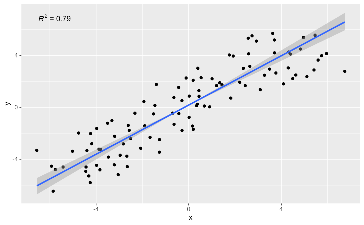
# using defaults (major axis regression)
ggplot(my.data, aes(x, y)) +
  geom_point() +
  stat_ma_line() +
  stat_ma_eq()


ggplot(my.data, aes(x, y)) +
  geom_point() +
  stat_ma_line() +
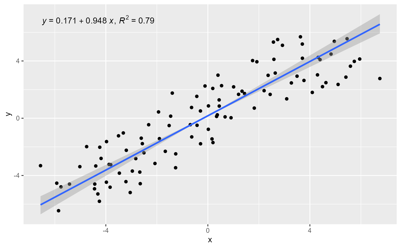
  stat_ma_eq(mapping = use_label("eq"))


ggplot(my.data, aes(x, y)) +
  geom_point() +
  stat_ma_line() +
  stat_ma_eq(mapping = use_label("eq"), decreasing = TRUE)


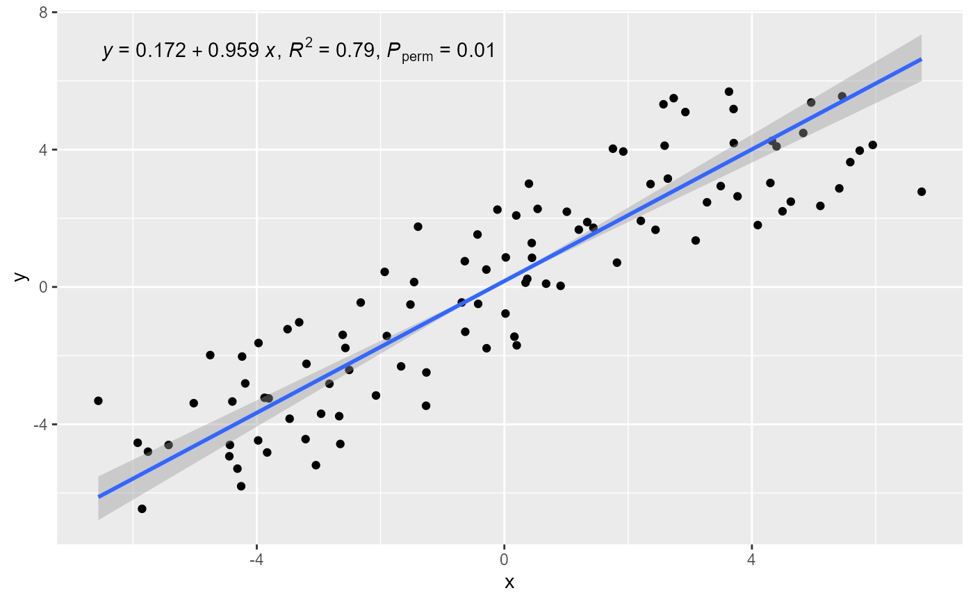
# use_label() can assemble and map a combined label
ggplot(my.data, aes(x, y)) +
  geom_point() +
  stat_ma_line(method = "MA") +
  stat_ma_eq(mapping = use_label("eq", "R2", "P"))


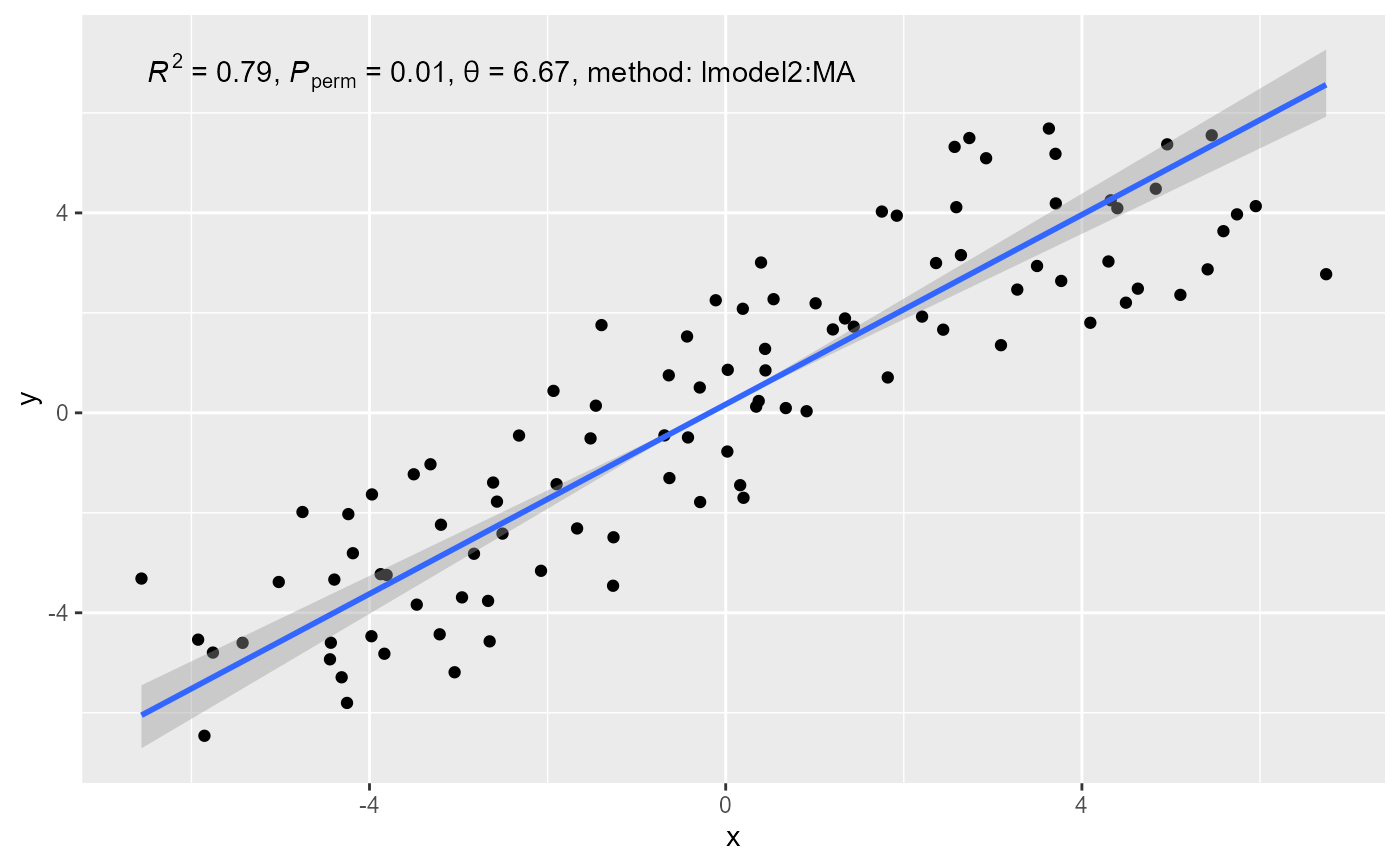
ggplot(my.data, aes(x, y)) +
  geom_point() +
  stat_ma_line(method = "MA") +
  stat_ma_eq(mapping = use_label("R2", "P", "theta", "method"))


# using ranged major axis regression
ggplot(my.data, aes(x, y)) +
  geom_point() +
  stat_ma_line(method = "RMA",
               range.y = "interval",
               range.x = "interval") +
  stat_ma_eq(mapping = use_label("eq", "R2", "P"),
             method = "RMA",
             range.y = "interval",
             range.x = "interval")


# No permutation-based test
ggplot(my.data, aes(x, y)) +
  geom_point() +
  stat_ma_line(method = "MA") +
  stat_ma_eq(mapping = use_label("eq", "R2"),
             method = "MA",
             nperm = 0)
#> No permutation test will be performed


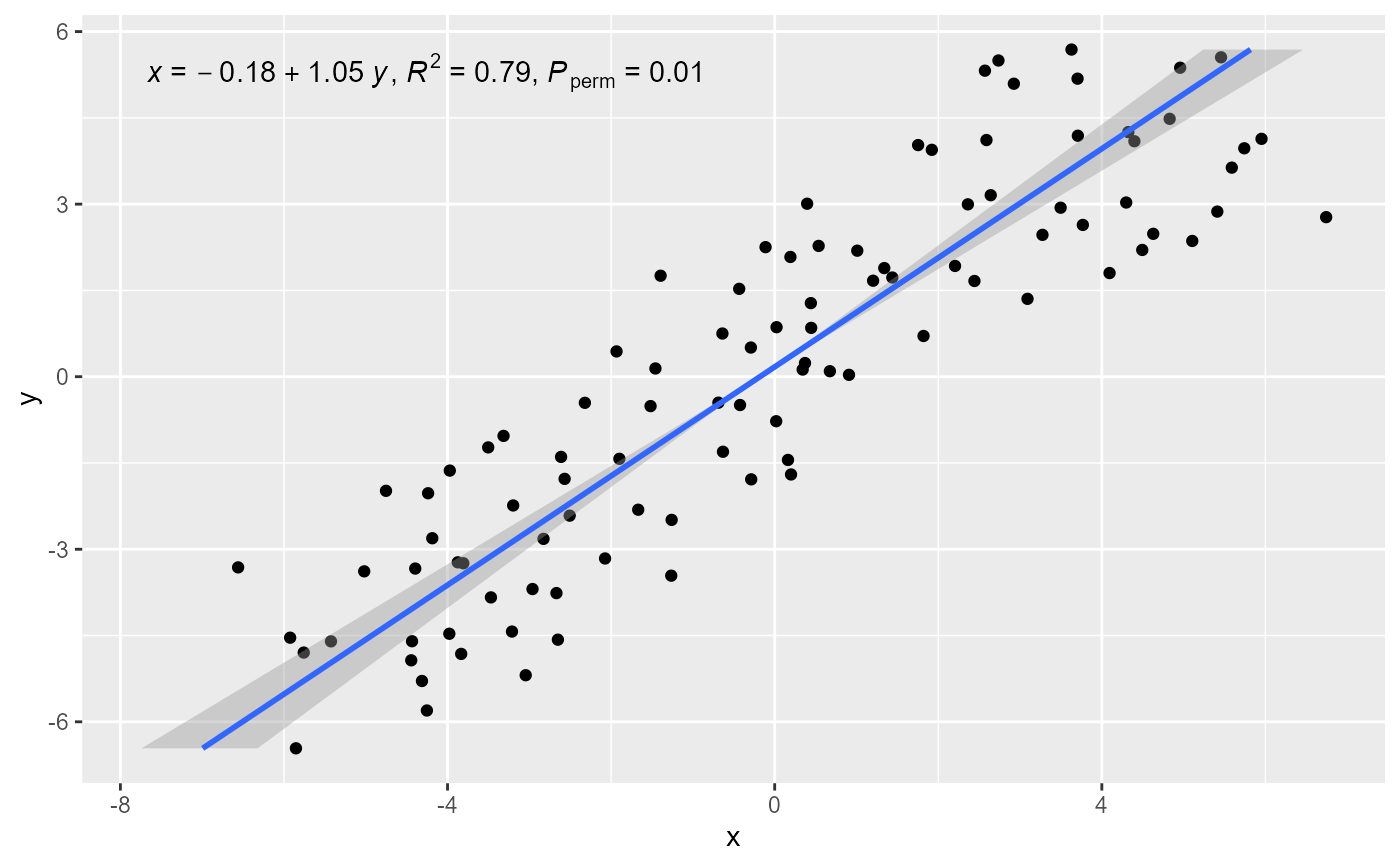
# explicit formula "x explained by y"
ggplot(my.data, aes(x, y)) +
  geom_point() +
  stat_ma_line(formula = x ~ y) +
  stat_ma_eq(formula = x ~ y,
             mapping = use_label("eq", "R2", "P"))


# modifying both variables within aes()
ggplot(my.data, aes(log(x + 10), log(y + 10))) +
  geom_point() +
  stat_poly_line() +
  stat_poly_eq(mapping = use_label("eq"),
               eq.x.rhs = "~~log(x+10)",
               eq.with.lhs = "log(y+10)~~`=`~~")


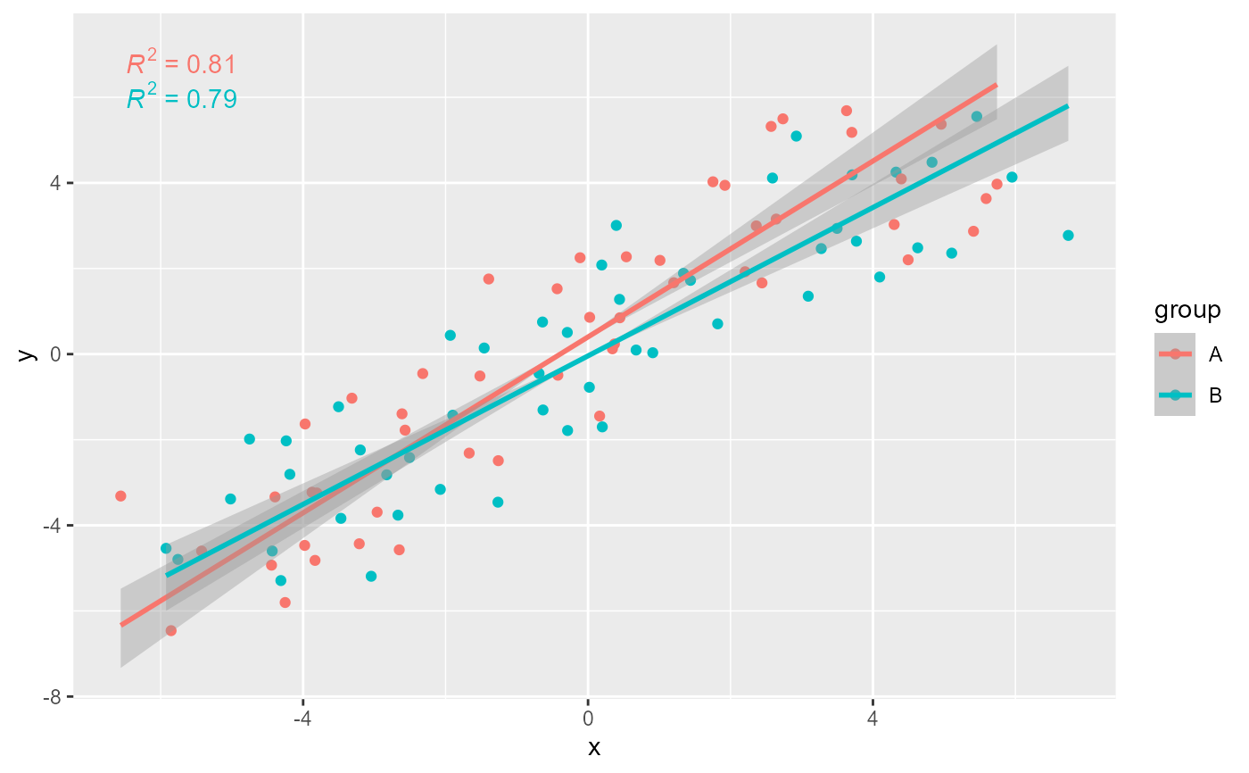
# grouping
ggplot(my.data, aes(x, y, color = group)) +
  geom_point() +
  stat_ma_line() +
  stat_ma_eq()


# labelling equations
ggplot(my.data,
       aes(x, y,  shape = group, linetype = group, grp.label = group)) +
  geom_point() +
  stat_ma_line(color = "black") +
  stat_ma_eq(mapping = use_label("grp", "eq", "R2")) +
  theme_classic()


# Inspecting the returned data using geom_debug_group()
# This provides a quick way of finding out the names of the variables that
# are available for mapping to aesthetics with after_stat().

gginnards.installed <- requireNamespace("gginnards", quietly = TRUE)

if (gginnards.installed)
  library(gginnards)

# default is output.type = "expression"
if (gginnards.installed)
  ggplot(my.data, aes(x, y)) +
    geom_point() +
    stat_ma_eq(geom = "debug_group")

#> [1] "PANEL 1; group(s) -1; 'draw_function()' input 'data' (head):"
#>                                 eq.label               rr.label
#> 1 italic(y)~`=`~0.171 + 0.948*~italic(x) italic(R)^2~`=`~"0.79"
#>                p.value.label              theta.label           n.label
#> 1 italic(P)[perm]~`=`~"0.01" italic(theta)~`=`~"6.67" italic(n)~`=`~100
#>   grp.label         method.label r.squared    theta p.value   n  fm.method
#> 1        -1 "method: lmodel2:MA" 0.7917998 6.665222    0.01 100 lmodel2:MA
#>   fm.class fm.formula fm.formula.chr        x npcx        y npcy PANEL group
#> 1  lmodel2      y ~ x          y ~ x -6.56061   NA 5.687505   NA     1    -1
#>                    label orientation
#> 1 italic(R)^2~`=`~"0.79"           x

if (FALSE) { # \dontrun{
if (gginnards.installed)
  ggplot(my.data, aes(x, y)) +
    geom_point() +
    stat_ma_eq(mapping = aes(label = after_stat(eq.label)),
               geom = "debug_group",
               output.type = "markdown")

if (gginnards.installed)
  ggplot(my.data, aes(x, y)) +
    geom_point() +
    stat_ma_eq(geom = "debug_group", output.type = "text")

if (gginnards.installed)
  ggplot(my.data, aes(x, y)) +
    geom_point() +
    stat_ma_eq(geom = "debug_group", output.type = "numeric")
} # }

Statistic	\(f\)	Supported model fit methods
`stat_poly_line()`	G	"lm", "rlm", "lts", "sma", "ma", "gls", others with methods `predict()` or `fitted()`
`stat_poly_eq()`	G	"lm", "rlm", "lts", "sma", "ma", "gls", others with needed accesors
`stat_quant_line()`	G	"rq", "rqss"
`stat_quant_band()`	G	"rq", "rqss"
`stat_quant_eq()`	G	"rq", "rqss"
`stat_ma_line()`	G	"SMA", "MA", "RMA", "OLS"
`stat_ma_eq()`	G	"SMA", "MA", "RMA", "OLS"
`stat_fit_residuals()`	G	"lm", "rlm", "lts", "sma", "ma", "gls", "rq", "rqss" others with method `residuals()`
`stat_fit_fitted()`	G	"lm", "rlm", "lts", "gls", "rq", "rqss" others with method `fitted()`
`stat_fit_deviations()`	G	"lm", "rlm", "lts", "gls", "rq", "rqss" others with methods `fitted()` and `weights()`
`stat_fit_augment()`	G	any with 'broom' method `augment()`
`stat_fit_glance()`	G	any with 'broom' method `glance()`
`stat_fit_tidy()`	G	any with 'broom' method `tidy()`
`stat_fit_tb()`	P	any with 'broom' method `tidy()`

Usage

Arguments

Value

Details

Variables returned by `stat_ma_line()`

Variables returned by `stat_ma_eq()`

Output types

Model formula and model fitting

Model equation label

Position of labels

Range of the prediction line

Model fit methods supported

See also

Aesthetics

Examples